[ home ]
13th Dec 2014: a better handout for students (PDF) and new results of 800+ rolls lower down the page. Still not significant!
10th Nov 2012: Thanks to reader Adam for pointing out a mistake with the chi-square goodness of fit test. I had the number of degrees of freedom wrong! I'm still interpreting the results as 'not proven' (scottish verdict), see below
Two classes, and 20 dice. Each student rolled two dice 10 or 12 times and recorded their results in a suitable table. We ended up with 164 recorded dice rolls (a few got lost in the tallying). You can download a spreadsheet in Libreoffice format with the results, graphs and the chi-square calculation.
To keep things simple, each student or pair of students had a pair of dice of contrasting colours. Once the results were recorded, they added the numbers on the two dice to produce the score, and tallied the results on the whiteboard (dry marker in one case and interactive in the other, final results recorded with mobile phone camera and whiteboard software).
Later in the lesson, the I developed the sample space diagram for two dice, and compared the scores with the results we found. I used that exercise to draw a distinction between the probability for each score predicted from the symmetry of the two plastic cubes, and the relative frequencies found from the actual experiment. In this page, I'll develop the mathematics step by step, but I may write this up as an 'investigation' lesson for my other classes.
Most textbooks suggest drawing the sample space diagram (aka possibility space diagram) for the totals of the scores on a green and a red dice.
| Sample space diagram for total score on two dice | ||||||
|---|---|---|---|---|---|---|
| + | 1 | 2 | 3 | 4 | 5 | 6 |
| 1 | 2 | 3 | 4 | 5 | 6 | 7 |
| 2 | 3 | 4 | 5 | 6 | 7 | 8 |
| 3 | 4 | 5 | 6 | 7 | 8 | 9 |
| 4 | 5 | 6 | 7 | 8 | 9 | 10 |
| 5 | 6 | 7 | 8 | 9 | 10 | 11 |
| 6 | 7 | 8 | 9 | 10 | 11 | 12 |
The most common score is 7 and scores 2 and 12 only appear once in the table. There are 36 outcomes, each of which has an equal chance of happening. So a frequency table can be drawn up and probabilities worked out...
| probabilities of scores | ||
|---|---|---|
| Score | Frequency | Probability |
| 2 | 1 | 1/36 |
| 3 | 2 | 2/36 |
| 4 | 3 | 3/36 |
| 5 | 4 | 4/36 |
| 6 | 5 | 5/36 |
| 7 | 6 | 6/36 |
| 8 | 5 | 5/36 |
| 9 | 4 | 4/36 |
| 10 | 3 | 3/36 |
| 11 | 2 | 2/36 |
| 12 | 1 | 1/36 |
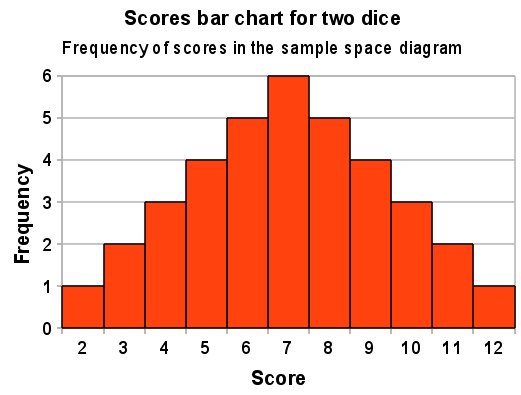
The bar chart below shows the distribution of the scores, more ways of scoring 7 and less ways of scoring 2 and 12. Asking for the expected frequency of (say) score 5 when you roll the two dice 72 times and 144 times will check that people understand the 'frequency' in this special case: its an expected frequency of that score for 36 rolls of two dice.
Below is the frequency table of the scores, the probability of the score calculated from the sample space diagram, and the expected frequency or 'expectation' as the textbook describes it. I've written the probabilities as decimals and rounded them to three decimal places.
| Rolling two dice and adding the scores | |||
|---|---|---|---|
| Score | Frequency | Probability | Expectation |
| 2 | 8 | 0.028 | 4.6 |
| 3 | 11 | 0.056 | 9.1 |
| 4 | 12 | 0.083 | 13.7 |
| 5 | 18 | 0.111 | 18.2 |
| 6 | 24 | 0.139 | 22.8 |
| 7 | 28 | 0.167 | 27.3 |
| 8 | 23 | 0.139 | 22.8 |
| 9 | 22 | 0.111 | 18.2 |
| 10 | 7 | 0.083 | 13.7 |
| 11 | 5 | 0.056 | 9.1 |
| 12 | 6 | 0.028 | 4.6 |
The 'expectation' column is found by multiplying each probability by the number of dice rolls (164). We had a discussion about the 'expected' values being decimal numbers. Its allowed!
Once you have the expected frequency or expectation of each score, it is natural to compare these to the observed frequencies using a frequency polygon. I'll be doing this in the next lesson, and encouraging students to describe the differences between the expected and observed frequencies.
Thanks to reader Adam for pointing out a mistake in this section, now corrected.
Using a 5% significance level, and 11 - 1 = 10 degrees of freedom, chi-square needs to be more than 18.31 (corresponding to p = 0.05) to reject the null hypothesis of no difference and less than 3.94 (corresponding to p = 0.95) to positively accept the null hypothesis of no difference. Below is a screen grab of the spreadsheet calculation of the chi-squared statistic. You can download the spreadsheet in Libreoffice format (.ods file).

Using an online statistical calculator (Kirkman T. W. 1996) provides a p value of 0.481 from this data which is higher than 0.05 so there is no significant difference between the observed and expected results. I maintain that we can't go forward and accept the hypothesis of no difference, as the p value is below 0.95. I dimly recollect that I am probably using a two tailed test, and perhaps should only be using a one tailed one. More revision needed here!
Another 71 rolls of two dice by 6 groups reveals observations that are further away from the expected values...

Adding these new scores into the original data set and using the online calculator yields
Chi-Squared: Results

The results of a X2 statistical test performed at 15:04 on 10-NOV-2012

11 data/expectation pairs (x,E):
( 12.0 , 6.500 ); ( 13.0 , 13.10 ); ( 13.0 , 19.60 ); ( 28.0 , 26.10 );
( 35.0 , 32.60 ); ( 45.0 , 39.20 ); ( 33.0 , 32.60 ); ( 31.0 , 26.10 );
( 11.0 , 19.60 ); ( 7.00 , 13.10 ); ( 7.00 , 6.500 );

chi-square = 15.6
degrees of freedom = 10
probability = 0.111
So the chi-square statistic has increased, but is still lower than 18.31, and the p value has decreased to 0.111 but is still higher than the 0.05 level we have set for rejecting the null hypothesis of no difference between expected and observed.

The new frequency polygon shows more differences near the peak, but the large differences between the expected and observed scores in the tails of the polygon contribute most to the higher chi-squared value.
All new results from 813 rolls of sets of two dice by 6 GCSE Maths classes summarised in the screen shot below
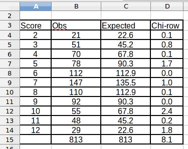
and the chi-square statistic and p-value calculated using the online calculator yields...
X2: Results

The results of a X2 statistical test performed at 08:42 on 14-DEC-2014

11 data/expectation pairs (x,E):
( 21.0 , 22.60 ); ( 51.0 , 45.20 ); ( 70.0 , 67.80 ); ( 78.0 , 90.30 ); ( 112. , 112.9 ); ( 147. , 135.5 ); ( 110. , 112.9 ); ( 92.0 , 90.30 ); ( 55.0 , 67.80 ); ( 48.0 , 45.20 ); ( 29.0 , 22.60 );

chi-square = 8.10
degrees of freedom = 10
probability = 0.619
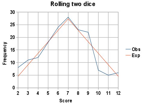
The p-value has increased but still not anywhere the 0.95 level needed to positively accept the hypothesis of no difference between observed and expected. Below is a graph comparing the observed (blue) and expected (red) frequencies...

The schemes of work for the GCSE in the two institutions I teach in are slightly different, so this topic comes up with two classes of 16-19 students in a month or so. They are saying that they want more group activities and games in the evaluations so I'll package this as an investigation along these lines
Keith Burnett, Last update: Sun Dec 14 2014